Plot Jz at a given time step

Use the Output parser to extract info of the time steps

Download Input files

• dipole_2d.data

• dipole_2d.post.xml

Setting up

Standard Loading of input, Parsing and Initializing RoxiePlotOutputs object

from roxieapi.commons.roxie_constants import PlotLabels
from roxieapi.commons.types import Plot2D
from roxieapi.output.parser import RoxieOutputParser
from roxieapi.output.plots import RoxiePlotOutputs

xml_file_path = "../input_files/eddy_currents.post.xml"
data_file_path = "../input_files/eddy_currents.data"

plots = RoxiePlotOutputs(xml_file_path, data_file_path)
parser = RoxieOutputParser(xml_file_path)

Show available plots of Eddy currents Time steps

# These are the possible things to plot on Mesh for eddy-currents
# Select one of the {pl}

for pl in PlotLabels.plotMesh2D_desc:
    lbl, _ = PlotLabels.lbl_desc_mesh2D(pl)
    print(f"Mesh Eddy plot '{pl}'   -    Label:  '{lbl}'")

Mesh Eddy plot '31'   -    Label:  'MUER'
Mesh Eddy plot '32'   -    Label:  '|BTOT|'
Mesh Eddy plot '34'   -    Label:  'AR'
Mesh Eddy plot '35'   -    Label:  'MUEFAC'
Mesh Eddy plot '75'   -    Label:  'Bx'
Mesh Eddy plot '76'   -    Label:  'By'
Mesh Eddy plot '121'   -    Label:  'JX'
Mesh Eddy plot '122'   -    Label:  'JY'
Mesh Eddy plot '123'   -    Label:  'JZ'
Mesh Eddy plot '124'   -    Label:  '|J|'
Mesh Eddy plot '125'   -    Label:  'J2S'
Mesh Eddy plot 'az'   -    Label:  'AZ'
Mesh Eddy plot 'norm_deriv_az'   -    Label:  'dAz/dn'
Mesh Eddy plot 'Bz'   -    Label:  'Bz'
Mesh Eddy plot 'jx'   -    Label:  'JX'
Mesh Eddy plot 'jy'   -    Label:  'JY'
Mesh Eddy plot 'jz'   -    Label:  'JZ'
Mesh Eddy plot 'j^2/sigma'   -    Label:  'J2S'
Mesh Eddy plot 'Hx'   -    Label:  'HX'
Mesh Eddy plot 'Hy'   -    Label:  'HY'
Mesh Eddy plot 'Hz'   -    Label:  'HZ'

In the above ROXIE file, we used 2 “Nsteps” (transient steps) and each one has 4 “Evaluation steps”

transient_steps = parser.opt[1].transient_steps_number
eddy_steps = parser.opt[1].step[1].eddy_steps_number

print(
    f"We have {transient_steps} transient steps, and each has {eddy_steps} eddy steps."
)

We have 2 transient steps, and each has 4 eddy steps.

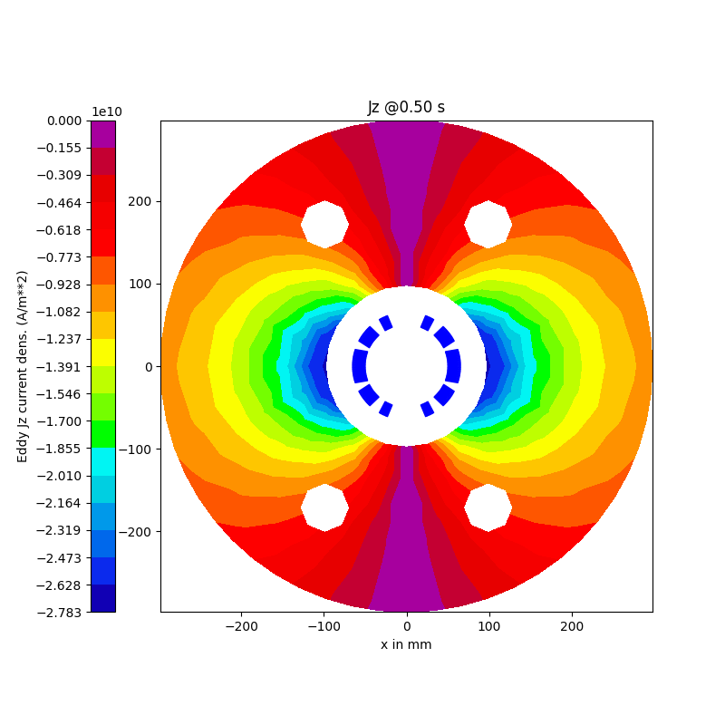
Let’s plot the current density during the excitation @ 4th eddy time step

snapshot_time = parser.opt[1].step[1].eddyTimeSteps[4].time
plot_created = Plot2D.create(f"Jz @{snapshot_time:.2f} s")

# Pass the selected {pl} to plot
plot_created.add_meshPlot("jz")

# Plot on 1st (optim) run, 2nd excitation (transient) step, 4th eddy time step
figure = plots.plots2d.plot_xs(plot_created, opt_step=1, trans_step=2, eddy_step=4)

# Eddy step is Optional, so below plot should be the same since the last (4-th) eddy step is used by default
figure = plots.plots2d.plot_xs(plot_created, opt_step=1, trans_step=2)

• 
•